Understanding how people behave on your website can be incredibly powerful for figuring out how to improve it.

There are of course many ways to try to do this, but finding patterns in behavioural data at scale via your analytics package holds many advantages. It can reveal common behaviours you’ve never considered, plus provide you with the basis to track these behaviours over time.

Unsupervised machine learning enables you to spot patterns in session-level data, and results in labelled sessions (i.e. which segment each session fits in) so that you can train a supervised machine learning algorithm to segment any session in the future.

In this blog post we will cover:

• A brief overview of how this works
• Detailed information about how to extract the required data from Google Analytics (with Python)
• Information about how to process it, such as commonly useful transformations (with Python)
• How to select the features for unsupervised machine learning (with Python)
• How to cluster the segments (with Python)
• How to finalise the segments (with Python)
• Next steps: training a natural network to classify any future session as belonging to a particular segment

A brief overview of how this works

See here for a more visual explanation, from a talk I delivered at MeasureFest.

Supervised machine learning uses labelled data to create a model that can be used to classify a new input, according to the labels it learned.

Unsupervised machine learning doesn’t use labelled data - it simply finds patterns in data. Essentially it can be used to find the labels.

This can be very useful for segmenting audiences.

To do this for visitors to your website, you can extract session IDs from your web analytics and multiple data points relating to what that person did within the session (such as the page they landed on, how long the spent per page, etc.), and then use an unsupervised machine learning algorithm to find patterns - giving us our behavioural segments.

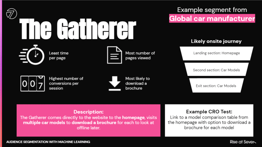
The results can be really interesting. The following is an example segment from a car manufacturer website:

Essentially, there is a group of users that come onto the website and ‘gather’ multiple brochures, and then take them offline to consume - they have the least amount of time per page (as they are just trying to get to the brochures) but the most pages per session as they navigate between the different car models. They download multiple brochures, so have the highest number of conversions per session.

It seems we can really improve this journey by having a section linked from the homepage (where they land) where they can download multiple car model brochures on one page. Worth a test!

So, how do we get these segments?

How to extract the required data from Google Analytics

There are two key routes to extracting the data from Google Analytics - you can either use BigQuery or the Google Analytics API.

We won’t cover extracting the relevant data from BigQuery in this blog post, but there are others that do.

We will cover using the Google Analytics API to extract session level data.

The first step to doing this is to enable the Google Analytics API and download your Client ID and Client secret. This is a good instructional post.

Once you have that done, you need to load in the relevant Python packages that you are going to need:

If there are any error messages, you will need to install the missing packages with pip.

This code then builds and executes the API call for you - as long as you replace [API FILE] with the path to your API details and [PROFILE ID] with the ID of the profile you want to extract data from:

Points to note:

• I have entered a dummy date for ‘startDate’ and ‘endDate’ - you will need to change this.
• I have also entered some dummy Metrics and Dimensions - you can change these (apart from clientId, which is necessary to get the data at the granular level that we need). Find useful Metrics and Dimensions here.
• There is a limit in terms of total Metrics and Dimensions you can pull in one go - a total of 10 across both.
• You are requesting data by ‘clientId’ - this can be the same user within a certain timeframe (it might be 90 days!), so you can often get some duplicate IDs. The data points you are pulling are generally session based though, so it will be the same user with different data points about their session each time.
• There are limits in terms of how many rows you can pull in one request (25,000) to get around this - particularly if you have lots of daily sessions! - you can create a loop to pull back data for each day individually and append on the bottom of a dataframe.
• If you have too many on a daily basis, you can even loop over a filter like device so that the request is under the limit and then merge after.
• You can also do the same to get around the Metric/Dimension limit - loop over different ones (keeping the ClientId each time) by day and then merge together.
• Remember that you can get multiple of the same clientId though - so to merge, you should concatenate with other data points to get a unique identifier for that individual session. For example, concatenate with the hour of the day they visited and the average time per page they sent to create a unique number.
• A way of getting a good sample of representative data throughout the year - but without having to pull data for the full 365 days - is to select random days to loop over. Otherwise seasonality may skew your segments.
• You can probably make do with around 50,000 sessions to work with for the clustering. We have used around 1 million before with Google Colab. Beyond this level, you will need more computation, likely via a Cloud provider.
• If you want to later train a neural network to classify any future session according to the segments you uncover, then you will need at least 500,000 sessions.

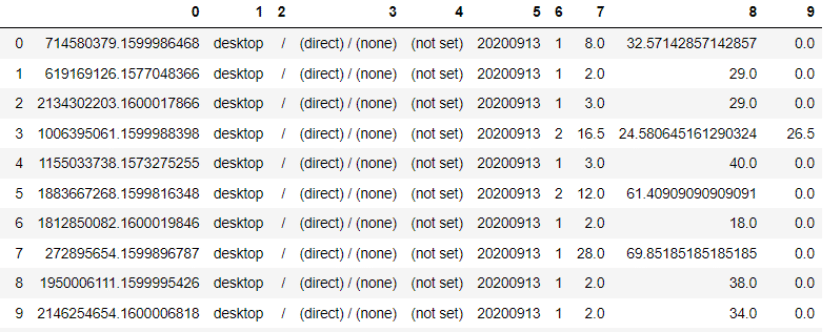
Once you have the data, it should look something like this:

Make sure you name the columns according to the Metrics and Dimensions that they represent. Here is a line of code to do that (change Metric1 etc. to the names of the Metrics/Dimensions you have called for):

Processing the data

Once you have the data, you need to prepare it for the unsupervised machine learning algorithm. This means transforming it to reduce dimensionality, plus making the format consistent for better performance of the algorithm.

Useful transformations

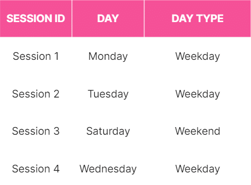
The first thing you will want to do is transform the data - mainly to reduce unnecessary noise later. For example, behaviour might not differ much between Monday, Tuesday, Wednesday, Thursday and Friday, but might really differ between weekdays and weekends as a whole. So, you may want to create a new column replacing Monday etc. with ‘Weekday’ and Saturday/Sunday with ‘Weekend’.

Here is the Python code to do that with Pandas (don’t forget to import it), if you have column in your dataframe called ‘Day’:

This will result in the following:

Other possible transformations include:

Change times of the day to morning/afternoon/evening/night. Here is the code to do that, if you have a column called ‘Hour’ from your original data:

Record when someone converts on a combination of two different data points, by adding an extra column with recording a value of ‘1’ when they hit both:

The following creates a new column called ‘Source-Organic’ from a ‘Source’ column (if you have extracted the Source for each session via the Google Analytics API) and then replaces all sources apart from the ones containing ‘organic’ with ‘not organic’. This is then useful for the next stage (One Hot Encoding, which we will get onto in a minute’):

Of course, this can be updated for any source.

There are also loads of other transformations you can do - such as combine the landing page and second page within a journey using concatenation, or replace the URL with the directory.

One hot encoding

The machine learning algorithm will only work with numbers, not text.

This causes issues for categorical variables - such as the source of the session.

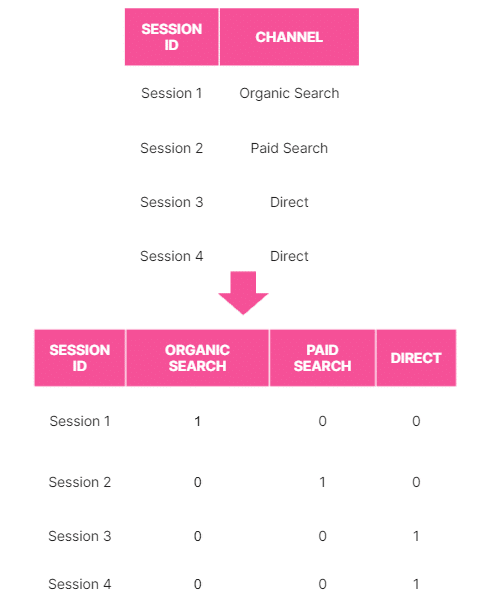
One hot encoding transforms categorical variables into numbers - but in such a way that won’t skew the machine learning algorithm.

So if you had three categories (say ‘Red’, ‘Green’, ‘Blue’) and you converted them into ascending numbers (say ‘1’, ‘2’, ‘3’) - then the machine learning algorithm would think the ‘Blue’ was ‘bigger’ than ‘Red’. This will cause problems.

One hot encoding solves this issue by converting categories into 1s and 0s in the following way:

Here is the code to convert a column with a categorical variable into columns with 1s and 0s:

Then you can add it back to the original dateframe (if that has been named as ‘df’):

Important point to note:

Ideally you want to put continuous/discrete variables (such as time per page) into ‘buckets’ too using transformations similar to those above and then use one hot encoding for those too. Otherwise it can skew the machine learning algorithm. At least test it!

Selecting the features

Now you have the data in a usable format, you should try to narrow down features that are going to be useful for clustering.

Firstly, you will have to use your common sense to some extent. What variables are likely to affect how a person behaves on the website - time of day (morning vs. evening?), where they land on the website, what source they came from?

Secondly, you can use something called ‘Best Subset Regression’ to help narrow down your choice - choosing various ‘explanatory’ variables and seeing how they relate to a ‘response’ variable. This will mean choosing a ‘response’ variable - what’s the ultimate behaviour that you want to differ in terms of output, based on inputs/features you are using to cluster? This could be revenue for example.

You then choose a selection of potential ‘explanatory’ variables (up to 10, otherwise your laptop may explode) and the model will try various combinations. Here’s the code:

I use this with various different explanatory variables and then use the ones that have consistently the lowest p-values (the value in the column P>|t| should be close to 0).

Clustering into segments

Now, you have session level data transformed to work with the algorithm, and an idea of which features you want to try to cluster on.

Next is to do the clustering itself. Firstly, load in the required packages:

Then, set a random seed - so that the results are repeatable:

Next, load in your data to cluster (having extracted and processed):

Next, you normalise the data set, using the features you narrowed down as being important in feature selection (then selecting them by column name - replacing what I have put in such as ‘Feature_Column1’ etc.):

Then you need to do Principal Component Analysis on the features. This potentially makes the clustering algorithm perform better by reducing the dimensionality of the data, whilst still retaining a lot of the information. You don’t really need to necessarily understand exactly why it’s important - but it’s definitely worth doing. Here’s the code:

Apply the K-means algorithm:

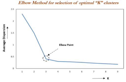
Finally, you want to assess how many clusters is the optimum number. To do this you want to use a silhouette score - which measures how far the K-means centroids are away from each other. Essentially, it measures how well-defined and differentiated the clusters are from each other. Here’s the code:

This will generate a graph. You want to choose the number of clusters that give an ‘elbow’ in the graph - beyond this point, gains from the score start to diminish:

Once you have the optimal number of clusters, you then run the algorithm with that number:

Finalising the Segments

Once you have the clusters (segments), you want to manually explore them - how different are they in terms of data points of interest? For example, based on the features you’ve selected such as time of day or traffic source, how different is the average order value?

You can get the mean for each data point of the clusters with the following:

This will help show the differences. You can then use something like a two sample T-Test (or Z-Test depending on the variable) to figure out how likely it is that the means are actually different between the segments - and not just the result of general fluctuation.

This is also when you interpret the clusters to determine what they are telling you in terms of behaviour. For example, 'The Gatherer' segment was quite obvious because of the different averages of the data points (least time on page, most conversions, most pages etc).

If the differences aren’t useful/interesting - try different features, a different number of clusters, etc.

Next Steps - Training a Neural Network to Classify Future Sessions

The next step is to train a neural network with your newly labelled data so that it can classify any future session on the website according to your segments. I’m not actually going to go into this now as we’ve covered a lot - but stay tuned, as I will be doing a follow up with this (and will link to it from here when it’s ready!).

Summary

• You can extract session level data from Google Analytics using the API
• Having done some initial processing of that data, you can then use an unsupervised machine learning algorithm to find interesting patterns, resulting in segments
• Once you have that you can train a neural network to classify any future session on the website according to the segments - I will go through this next time